【理论】object detection api调参详解(兼SSD算法参数详解) |
您所在的位置:网站首页 › borrow rate理论 › 【理论】object detection api调参详解(兼SSD算法参数详解) |
【理论】object detection api调参详解(兼SSD算法参数详解)
|
一、引言 使用谷歌提供的object detection api图像识别框架,我们可以很方便地重新训练一个预训练模型,用于自己的具体业务。以我所使用的ssd_mobilenet_v1预训练模型为例,训练所需参数都在training文件夹下的ssd_mobilenet_v1_coco.config中预先配置了,只需对少量路径参数做修改即可。
但是这种“傻瓜式”的训练参数配置方法有很大不足。一是无法理解训练参数背后的原理,不利于技术积累;二是一旦遇到需要优化的问题时,不知道如何调整训练参数。例如,我使用默认配置的训练参数对模型进行长期训练后,发现模型始终无法收敛,loss值一直在3~5的范围内波动,没有继续下降。但在没有弄清楚训练参数如何调整之前,我一直没能解决该问题。
所以,我们必须弄清楚每个训练参数的出处、含义、数值调整范围,才能自行对训练文件做合理配置,从而灵活解决各类训练问题。
本文以ssd_mobilenet_v1预训练模型为例,详细解释其训练参数的含义及调整范围。对其它预训练模型的训练参数的分析方法类似,不再逐一展开。
二、正文 首先简单解释一下,object_detection api框架将训练参数的配置、参数的可配置数值的声明、参数类的定义,分开放置在不同文件夹里。训练参数的配置放在了training文件夹下的.config文件中,参数的可配置数值的声明写在了protos文件夹下对应参数名的.proto文件中,参数类的定义则放在了object_detection总文件夹下对应参数名的子文件夹里或者是core文件夹里。
.config文件里包含5个部分:model, train_config, train_input_reader, eval_config, eval_input_reader。以ssd_mobilenet_v1_pets.config为例,打开该文件,按照从上到下、从外层到内层的顺序,依次解释各训练参数。
2.1 model{ } 包含了ssd{ }。
2.1.1 ssd { } 包含了SSD算法使用的各类训练参数。从2.1.2开始逐个展开解释。
2.1.2 num_classes 分类数目。例如,我要把所有待检测目标区分成6类,则这里写6。
2.1.3 box_coder、faster_rcnn_box_coder box_coder { faster_rcnn_box_coder { y_scale: 10.0 x_scale: 10.0 height_scale: 5.0 width_scale: 5.0 } }
这部分参数用于设置box编解码的方式。可选参数值: FasterRcnnBoxCoder faster_rcnn_box_coder = 1; MeanStddevBoxCoder mean_stddev_box_coder = 2; SquareBoxCoder square_box_coder = 3; KeypointBoxCoder keypoint_box_coder = 4;
SSD算法借鉴了Faster-RCNN的思想,所以这里的设置应该选faster_rcnn_box_coder。
Faster-RCNN中,bounding box的坐标值可以用两种不同的坐标系表示:一种坐标系以图片左上角作为原点,我称其为绝对坐标系;另一种坐标系以用于参考的anchor boxes的中心点位置作为原点,我称其为相对坐标系。
所谓box编码就是以anchor box为参照系,将box的绝对坐标值和绝对尺寸,转换为相对于anchor box的坐标值和尺寸。所谓box解码就是将box的相对坐标值和相对尺寸,转换回绝对坐标值和绝对尺寸。
在SSD算法中,anchor box的概念被叫做default box。box编解码中的box,则是指预测框(predicted box,也叫做bounding box)和真实框(ground-truth box)。SSD中的box编码,就是以default box为参照系,将predicted box和ground-truth box转换为用相对于default box的数值来表示;SSD中的box解码,则是将predicted box和ground-truth box转换回用绝对坐标系数值表示。
faster_rcnn_box_coder的解释详见box_coders文件夹下的faster_rcnn_box_coder.py。重点分析这组转换公式即可: ty = (y - ya) / ha tx = (x - xa) / wa th = log(h / ha) tw = log(w / wa) ( x, y, w, h是待编码box的中心点坐标值、宽、高;xa, ya, wa, ha是anchor box的中心点坐标值、宽、高; tx, ty, tw, th则是编码后的相对中心点坐标值、宽、高。在转换中用除法实现了归一化)
此处的y_scale、x_scale、height_scale、width_scale则是对ty、tx、th、tw的放大比率。
2.1.4 matcher、argmax_matcher matcher { argmax_matcher { matched_threshold: 0.5 unmatched_threshold: 0.5 ignore_thresholds: false negatives_lower_than_unmatched: true force_match_for_each_row: true } }
这部分参数用于设置default box和ground-truth box之间的匹配策略。
可选参数值: ArgMaxMatcher argmax_matcher = 1; BipartiteMatcher bipartite_matcher = 2;
SSD算法中,采用了ArgMaxMatcher策略,所以这里选择argmax_matcher。所谓ArgMaxMatcher策略,就是选取最大值策略。在matchers文件夹的argmax_matcher.py里有详细解释。
在SSD算法中,用default box和ground-truth box的IOU值(一种定量的相似度)来作为阈值标准,设置了matched_threshold、unmatched_threshold两个阈值。分为三种子情况: (1) 当IOU >= matched_threshold时:default box和ground-truth box匹配,default box记为正样本。 (2) 当IOU < unmatched_threshold时:default box和ground-truth box不匹配。引入另一个参数negatives_lower_than_unmatched。negatives_lower_than_unmatched=true时:所有不匹配default box记为负样本;negatives_lower_than_unmatched=false时:所有不匹配default box被忽略。 (3) 当matched_threshold > IOU >= matched_threshold时:记为中间态,并引入另一个参数negatives_lower_than_unmatched。negatives_lower_than_unmatched=true时:所有中间态default box被忽略;negatives_lower_than_unmatched=false时:所有中间态default box被记为负样本。上述参数例中两个阈值都是0.5,故没有中间态。
ignore_thresholds: 没有找到具体解释。应该是显式地指定是否单独设置ignore阈值。
force_match_for_each_row:设置为true,以确保每个ground-truth box都至少有一个default box与之对应,防止有些ground-truth没有default box对应。否则,这些ground-truth box最后将没有bounding box回归对应,也就是产生了漏检。
在SSD算法中,将所有ground-truth box按行排列、将所有default box按列排列,形成一个矩阵。矩阵的每一格记录ground-truth box和default box的匹配结果。匹配分两步: (1) 对每行的ground-truth box,采用ArgMax策略,选择与它的IOU最大的default box进行匹配; (2) 对剩余的每一个没有匹配到ground-truth box的default box,选择所有与它的IOU大于match threshold的ground-truth box进行匹配。
这样,每个ground-truth box至少有一个default box与它匹配。
2.1.5 similarity_calculator、iou_similarity similarity_calculator { iou_similarity { } }
这个参数选择使用何种相似度计算标准。在匹配过程中,用default box和ground-truth box的相似度来判断二者是否匹配。在2.1.4小节中,已经解释了SSD算法是采用IOU值来定量衡量相似度的,故这里选择数值iou_similarity。
2.1.6 anchor_generator、ssd_anchor_generator anchor_generator { ssd_anchor_generator { num_layers: 6 min_scale: 0.2 max_scale: 0.95 aspect_ratios: 1.0 aspect_ratios: 2.0 aspect_ratios: 0.5 aspect_ratios: 3.0 aspect_ratios: 0.3333 } }
这部分选择anchor box的生成器(一组生成公式),配置了生成器所需的部分参数。
Anchor box的生成器可以有如下选择: GridAnchorGenerator grid_anchor_generator = 1; SsdAnchorGenerator ssd_anchor_generator = 2; MultiscaleAnchorGenerator multiscale_anchor_generator = 3;
ssd_anchor_generator这部分设置了生成default box所需的一些参数。详细解释可参考SSD的论文。这里只解释一下各参数的基本含义。
num_layers: 数值为6,代表提取特征用的6个层。SSD算法借鉴了特征金字塔的思想,从6个feature map层同步提取特征。
min_scale和max_scale:我目前的理解是:scale是同层的default boxes中的小正方形宽相对于resize的输入图像宽的比率。在SSD论文中,min_scale是指该比率在最低层feature map的值,max_scale是指该比率在最高层feature map的值。至于中间4层feature map上的比率值,论文中是以线性插值的方式来获得的(但参考代码中不是这样确定各层比率的)。
aspect_ratios:指定了同一个feature map层上的default box的宽长比。例如,这里aspect ratios指定了5种宽长比,利用图1的公式(Sk: scale*resize width; ar: aspect_ratios)可以计算出6种不同宽长的default boxes(包括2种正方形、4种长方形)。注意:某些feature map层不使用3和1/3这一对aspect_ratios,故只生成4个default boxes。详细解释可参考SSD的论文。
2.1.7 image_resizer、fixed_shape_resizer image_resizer { fixed_shape_resizer { height: 300 width: 300 } }
这部分参数设置了对输入图像的resize策略。可选参数: KeepAspectRatioResizer keep_aspect_ratio_resizer = 1; FixedShapeResizer fixed_shape_resizer = 2;
传统SSD300模型中,输入图像被统一resize为300*300。故这里选择fixed_shape_resizer,且height和width均设置为300。
2.1.8 box_predictor box_predictor { convolutional_box_predictor { min_depth: 0 max_depth: 0 num_layers_before_predictor: 0 use_dropout: false dropout_keep_probability: 0.8 kernel_size: 1 box_code_size: 4 apply_sigmoid_to_scores: false conv_hyperparams { activation: RELU_6, regularizer { l2_regularizer { weight: 0.00004 } } initializer { truncated_normal_initializer { stddev: 0.03 mean: 0.0 } } batch_norm { train: true, scale: true, center: true, decay: 0.9997, epsilon: 0.001, } } } }
这部分设置了预测器相关层的参数。
关于Box predictor的解释详见core文件夹下的box_predictor.py。Box predictors输入高层的feature map,输出两类预测:(1)编码后的predicted box的相对位置;(2)predicted box里的物体类别。
Box predictor的可选参数范围: ConvolutionalBoxPredictor convolutional_box_predictor = 1; MaskRCNNBoxPredictor mask_rcnn_box_predictor = 2; RfcnBoxPredictor rfcn_box_predictor = 3; WeightSharedConvolutionalBoxPredictor weight_shared_convolutional_box_predictor = 4;
这些参数值的具体定义详见predictors文件夹。这里选用了convolutional_box_predictor,其含义是在所有feature maps后额外增加一个中间1x1卷积层。选择原因不明。
关于convolutional_box_predictor{ }内的许多参数的含义及数值范围,详见protos文件夹下的box_predictor.proto文件。下面逐个简单说明一下。
min_depth和max_depth:在位置回归和类别检测之前额外插入的feature map层深度的最小值和最大值。当max_depth=0时,表示在位置回归和类别检测之前,额外插入的feature map层数=0。
num_layers_before_predictor:在检测器之前的额外convolutional层的层数。
use_dropout:对class prediction是否使用dropout来防止过拟合。
dropout_keep_probability:如果使用了dropout,dropout的数值保留概率。
kernel_size:最后的卷积核的尺寸。
box_code_size:我的理解是box需要编码的参数个数。SSD算法里是cx, cy, w, h这4个参数需要编码,所以box_code_size=4。
apply_sigmoid_to_scores:最后class prediction输出时是否采用sigmoid。
conv_hyperparams{ }:卷积操作超参数的设置。详见protos文件夹里的hyperparams.proto。
activation:激活函数。目前可以选择NONE、RELU、RELU_6。这里选择了RELU_6。关于激活函数的细节,请自行查阅资料。
regularizer:正则化操作。目前可以选择l1_regularizer、l2_regularizer。这里选择了l2_regularizer。例子里L2_regularizer的weight值只有0.00004,所以正则化操作对loss的影响较小。关于L1正则化、L2正则化的细节,请自行查阅资料。
Initializer{ }:随机数初始化机制设置。可选参数如下: TruncatedNormalInitializer truncated_normal_initializer = 1; VarianceScalingInitializer variance_scaling_initializer = 2; RandomNormalInitializer random_normal_initializer = 3; 这里选择了truncated_normal_initializer。
truncated_normal_initializer:截断的正态分布随机数初始化机制。如果数值超过mean两个stddev,则丢弃。
batch_norm{ }:关于Batch Normalization(批标准化)的一些参数设置。Batch Normalization可以强制将输入激活函数的数值分布拉回标准正态分布,以防止训练过程中产生反向梯度消失,加速训练收敛。批标准化中会用到两个参数γ和β,分别定量化缩放和平移操作。细节请自行参阅相关资料。这里解释一下batch_norm的一些参数:: train: true——如果为true,则在训练过程中batch norm变量的值会更新,也就是得到了训练。如果为false,则在训练过程中batch norm变量的值不会更新。 scale: true——如果为true,则乘以γ;如果为false,则不使用γ。 center: true——如果为true,则加上β的偏移量;如果为false,则忽略β。 decay: 0.9997——衰减率。作用存疑。 epsilon: 0.001——添加到方差的小浮点数,以避免除以零。
2.1.9 feature_extractor feature_extractor { type: 'ssd_mobilenet_v1' min_depth: 16 depth_multiplier: 1.0 conv_hyperparams { activation: RELU_6, regularizer { l2_regularizer { weight: 0.00004 } } initializer { truncated_normal_initializer { stddev: 0.03 mean: 0.0 } } batch_norm { train: true, scale: true, center: true, decay: 0.9997, epsilon: 0.001, } } }
这部分设置了特征提取器相关层的参数。
不同模型的feature extractor的基类定义,详见meta_architectures文件夹下的对应文件。例如SSD模型的SSDFeatureExtractor基类,定义在meta_architectures文件夹下的ssd_meta_arch.py文件里。
不同预训练模型的feature extractor的类定义,详见models文件夹下的对应文件。例如ssd_mobilenet_v1预训练模型的feature extractor类,定义在models文件夹下的 ssd_mobilenet_v1_feature_extractor.py文件里。
models文件夹下的feature extractor类,是meta_architectures文件夹下的feature extractor基类的子类。
下面解释一下相关参数。 type:例子中使用了预训练模型ssd_moiblenet_v1的feature_extractor,所以这里填写'ssd_mobilenet_v1'。
min_depth:最小的特征提取器的深度。这里填16。原因不明。
depth_multiplier:是施加在每个input通道上的卷积核的数目。用于计算深度卷积分离后的输出通道总数。这里是一个浮点数。
conv_hyperparams超参数的含义和配置同2.1.8小节,不再重复解释。
2.1.10 loss loss { classification_loss { weighted_sigmoid { } } localization_loss { weighted_smooth_l1 { } } hard_example_miner { num_hard_examples: 3000 iou_threshold: 0.99 loss_type: CLASSIFICATION max_negatives_per_positive: 3 min_negatives_per_image: 0 } classification_weight: 1.0 localization_weight: 1.0 }
这部分设置了损失函数loss相关的参数。
loss{ }可选参数: // Localization loss to use. optional LocalizationLoss localization_loss = 1; // Classification loss to use. optional ClassificationLoss classification_loss = 2; // If not left to default, applies hard example mining. optional HardExampleMiner hard_example_miner = 3; // Classification loss weight. optional float classification_weight = 4 [default=1.0]; // Localization loss weight. optional float localization_weight = 5 [default=1.0]; // If not left to default, applies random example sampling. optional RandomExampleSampler random_example_sampler = 6;
SSD算法的loss分为目标分类损失函数(classification loss)和目标位置损失函数(localization loss),loss公式详见SSD论文。SSD算法也使用了某种难样本挖掘策略用于平衡正负样本比例。所以这里设置了classification_loss、localization_loss、hard_example_miner、classification_weight、localization_weight这5个参数。
下面解释一下这5个参数的具体配置。
classification_loss:可选参数: WeightedSigmoidClassificationLoss weighted_sigmoid = 1; WeightedSoftmaxClassificationLoss weighted_softmax = 2; WeightedSoftmaxClassificationAgainstLogitsLoss weighted_logits_softmax = 5; BootstrappedSigmoidClassificationLoss bootstrapped_sigmoid = 3; SigmoidFocalClassificationLoss weighted_sigmoid_focal = 4; 定义了分类输出的激活函数。具体含义请自行查阅资料。这里的设置和前面Box predictor部分的apply_sigmoid_to_scores设置是否有冲突,暂时没能确认。
localization_loss:可选参数: WeightedL2LocalizationLoss weighted_l2 = 1; WeightedSmoothL1LocalizationLoss weighted_smooth_l1 = 2; WeightedIOULocalizationLoss weighted_iou = 3; 定义了用于localization loss的正则化方法。具体含义请自行查阅资料。这里的设置和前面Box predictor部分的正则化设置是否有冲突,暂时没能确认。
hard_example_miner:难样本挖掘策略。SSD算法随机抽取一定数量的负样本(背景位置的default boxes),按一定规则进行降序排列,选择前k个作为训练用负样本,以保证训练时的正负样本比例接近1:3。下面解释一下它的具体子参数含义。 num_hard_examples: 3000——难样本数目。 iou_threshold: 0.99——在NMS(非极大抑制)阶段,如果一个example的IOU值比此阈值低,则丢弃。 loss_type: CLASSIFICATION——挖掘策略是否只使用classification loss,或只使用localization loss,或都使用。可选参数: BOTH = 0; (缺省选择?) CLASSIFICATION = 1; (缺省选择?) LOCALIZATION = 2; max_negatives_per_positive: 3——每1个正样本对应的最大负样本数。 min_negatives_per_image: 0——如何设置存疑。我目前的理解:在图片没有正样本的极端情况下,如果把这个值设置为一个正数,可以避免模型在图片上检测出目标来,防止了误检出。
classification_weight:用于配置classifiation loss在总loss中的权重。
localization_weight:用于配置localization loss在总loss中的权重。
2.1.11 normalize_loss_by_num_matches 我的理解:如果选true,则根据匹配的样本数目归一化总loss,也就是总loss公式中,用加权的classification loss和加权的localization loss计算出总loss后,还要再除以一个正样本总数N。如果选false,则计算出总loss后,不用再除以正样本总数N。
2.1.12 post_processing post_processing { batch_non_max_suppression { score_threshold: 1e-8 iou_threshold: 0.6 max_detections_per_class: 100 max_total_detections: 100 } score_converter: SIGMOID }
这部分配置了SSD算法的后处理阶段的参数。下面逐一解释。
batch_non_max_suppression{ }:这部分配置了批次的NMS(非极大抑制)策略的参数。先简单解释下NMS策略的目的。以目标检测为例,在最后阶段,一个目标上可能有很多个bounding box,但是最终目标检测框只有一个。因此,我们可以用NMS策略,逐次过滤掉其余的bounding box,最终只保留一个bounding box作为结果。关于NMS算法请自行参阅相关资料。下面简单解释一下具体参数含义: score_threshold: 1e-8——分数低于此阈值的box被过滤掉(去除非极大分数的)。 iou_threshold: 0.6——和之前选择的box的IOU值超过此阈值的box被过滤掉(去除重叠度高的) max_detections_per_class: 100——每个类别可保留的检测框的最大数目。 max_total_detections: 100——所有类别可保留的检测框的最大数目。
score_converter:检测分数的转换器类型选择。可选参数: // Input scores equals output scores. IDENTITY = 0; // Applies a sigmoid on input scores. SIGMOID = 1; // Applies a softmax on input scores. SOFTMAX = 2;
2.2 train_config{ } 训练用参数的配置。详见protos文件夹下的train.proto。下面解释.config例中的参数。
2.2.1 batch_size 每个批次的训练样本数。一般是2的幂次方。我只有CPU资源,所以batch_size设置比较小。
2.2.2 optimizer{ } 优化器的参数配置部分。
由于优化器的配置很关键,所以这部分想更详细展开一些。首先介绍一下参数的含义及可选范围,然后分别贴两个优化器配置的例子。
目前可选的优化器参数: RMSPropOptimizer rms_prop_optimizer MomentumOptimizer momentum_optimizer AdamOptimizer adam_optimizer 关于这三种优化器的特性,可自行参阅相关资料。
rms_prop_optimizer的可选参数: LearningRate learning_rate = 1; float momentum_optimizer_value = 2 [default = 0.9]; float decay = 3 [default = 0.9]; float epsilon = 4 [default = 1.0];
momentum_optimizer的可选参数: LearningRate learning_rate = 1; float momentum_optimizer_value = 2 [default = 0.9];
adam_optimizer的可选参数: LearningRate learning_rate = 1;
学习率learning_rate的可选参数: ConstantLearningRate constant_learning_rate = 1; ExponentialDecayLearningRate exponential_decay_learning_rate = 2; ManualStepLearningRate manual_step_learning_rate = 3; CosineDecayLearningRate cosine_decay_learning_rate = 4; 解释如下: constant_learning_rate:恒定学习率。恒定学习率太小则收敛很慢;太大则在极值附近震荡难以收敛。故一般不会使用。 exponential_decay_learning_rate:学习率按照指数规律衰减。下面会展开并举例(例1)。 manual_step_learning_rate:学习率按照人工设置的step逐段变小。下面会展开并举例(例2)。 cosine_decay_learning_rate:学习率按照噪声线性余弦规律衰减。
exponential_decay_learning_rate可选参数: float initial_learning_rate [default = 0.002]; uint32 decay_steps [default = 4000000]; float decay_factor [default = 0.95]; bool staircase [default = true]; float burnin_learning_rate [default = 0.0]; uint32 burnin_steps [default = 0]; float min_learning_rate [default = 0.0]; 简单解释如下: initial_learning_rate:初始学习率数值。 decay_steps:衰减周期。即每隔decay_steps步衰减一次学习率。下面例1中写的是800720步,而总的训练步数不过才200000步,显然decay_steps的设置偏大了,导致在整个训练过程中,学习率实际上没有任何指数衰减。这个设置不合理。 decay_factor:每次衰减的衰减率。 staircase:是否阶梯性更新学习率,也就是每次衰减结果是向下取整还是float型。 burnin_learning_rate:采用burnin策略进行调整的学习率(初始值?)。SSD算法中,是否有burnin策略、buinin策略又是如何调整学习率的,目前我还不太清楚。存疑。参考:在yolov3所用的darknet中,当学习率更新次数小于burnin参数时,学习率从小到大变化;当更新次数大于burnin参数后,学习率按照配置的衰减策略从大到小变化。 burnin_steps:按照字面意思,是burnin策略的调整周期。即每隔burnin_steps步调整一次burnin_learning_rate。 min_learning_rate:最小学习率。采用衰减策略变小的学习率不能小于该值。
manual_step_learning_rate可选参数: float initial_learning_rate = 1 [default = 0.002]; message LearningRateSchedule { optional uint32 step = 1; optional float learning_rate = 2 [default = 0.002]; } repeated LearningRateSchedule schedule = 2; optional bool warmup = 3 [default = false]; 简单解释如下: initial_learning_rate:初始学习率数值。 schedule:人工规划策略。包含两个参数: step——当前阶梯从全局的第step步开始。 learning_rate——当前阶梯的学习率。 warmup:对于全局步数区间[0, schedule.step]之间的steps,是否采用线性插值法来确定steps对应的学习率。缺省是false。
优化器还有3个独立参数: momentum_optimizer_value: momentum超参数。通过引入这个超参数(公式中一般记为γ),可以使得优化在梯度方向不变的维度上的更新速度变快,在梯度方向有所改变的维度上的更新速度变慢,从而加快收敛并减小震荡。 decay:衰减率。含义和出处不明。 epsilon:可能是迭代终止条件。
优化器配置例1: 优化器使用rms_prop_optimizer。 采用指数衰减策略来调整学习率。 optimizer { rms_prop_optimizer: { learning_rate: { exponential_decay_learning_rate { initial_learning_rate: 0.0001 decay_steps: 800720 decay_factor: 0.95 } } momentum_optimizer_value: 0.9 decay: 0.9 epsilon: 1.0 } }
优化器配置例2: 优化器使用momentum_optimizer。 采用人工设置下降阶梯的策略来调整学习率。 use_moving_average:设为false表示保存模型参数时,不使用moving average策略。moving average(移动平均)是一种保存模型参数的策略,会对不同迭代次数的模型的参数进行平均后再保存。 optimizer { momentum_optimizer: { learning_rate: { manual_step_learning_rate { initial_learning_rate: 0.0002 schedule { step: 1 learning_rate: .0002 } schedule { step: 900000 learning_rate: .00002 } schedule { step: 1200000 learning_rate: .000002 } } } momentum_optimizer_value: 0.9 } use_moving_average: false }
2.2.3 fine_tune_checkpoint 用于设置预训练模型的参数文件model.ckpt的路径。该参数文件用于精调。当训练开始时,导入已预训练好的模型参数,可以缩短训练过程。从零开始训练时,由于没有预训练模型的参数文件,故可以屏蔽这个路径参数。
2.2.4 from_detection_checkpoint 此参数已被废弃,使用fine_tune_checkpoint_type替代。
fine_tune_checkpoint_type:用来确定fine tune checkpoint使用的是分类模型参数还是检测模型参数。可选参数值:“”,“classification”,“detection”。
2.2.5 load_all_detection_checkpoint_vars 用于确定是否导入所有和模型变量名字和大小相符的detection checkpoint变量。只在使用检测模型时有效。
2.2.6 num_steps 训练总步数。如果设置为0,则训练步数为无穷大。
2.2.7 data_augmentation_options 数据增强参数配置。可选参数详见protos文件夹下的preprocessor.proto。 这个例子里数据增强使用了两个具体参数: random_horizontal_flip——随机水平翻转。 ssd_random_crop——SSD算法图像随机裁剪。
2.3 train_input_reader{ } 训练集数据的路径配置。可选参数详见protos文件夹下的input_reader.proto。
2.3.1 tf_record_input_reader、input_path 训练用tf_record格式数据集的路径配置。
2.3.2 label_map_path labelmap.pbtxt文件的路径配置。labelmap.pbtxt文件定义了待分类目标的id号和标签名称之间的映射关系。
2.4 eval_config{ } 测试用参数的配置。可选参数详见protos文件夹下的eval.proto。
2.4.1 metrics_set 用于配置评估模型性能的标准。 可选参数详见框架总目录下eval_util.py里的EVAL_METRICS_CLASS_DICT。目前有8种。 例子中使用的是coco_detection_metrics, 是使用coco数据集进行目标检测时评估模型性能的标准。
2.4.2 num_examples 测试样本数目。
2.5 eval_input_reader{ } 测试集数据的路径配置。可选参数详见protos文件夹下的input_reader.proto。
2.5.1 tf_record_input_reader、input_path 测试用tf_record格式数据集的路径配置。
2.5.2 label_map_path 同2.3.2节。
2.5.3 shuffle 随机排序操作配置。如果选false,则对测试样本不进行随机排序操作。
2.5.4 num_readers 用于配置可并行读入的文件分片的数目。 |
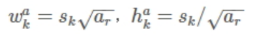 图1——default box宽长计算公式
【本文地址】
今日新闻 |
推荐新闻 |